Post-processing simulations¶

pytrnsys post-processes TRNSYS simulations based on configuration files with the extension .config, just like when running them.

Note

The configuration file does not require a header. It should contain different keyword commands on single lines. Comments start with # characters. End of line comments are possbile.

The existing commands are listed per topic in the following.

Generic¶

typeOfProcess (string, default ‘completeFolder’)

This parameter defines how data is processed. There are various possible arguments:

‘completeFolder’: Identifies data sets through lst files in pathBase and its subfolders.
‘individual’: Only the specified files will be processed. With timeBase specifying the time steps in the file (monthly, daily, hourly, or timeStep for a user-defined time base) and dataFolder the path to the file, which needs to be defined somewhere else in the config file, the files are specified like:
```
stringArray fileToLoad "timeBase" "dataFolder" "fileName"
```
‘casesDefined’: TBD
‘citiesFolder’: Data sets are defined by subfolders in pathBase, which are named according to the cities parameter.
‘config’: TBD
‘json’: Identifies data sets through json files in pathBase and its subfolders. Can also be used on -results.json files.

processParallel (bool, default True)

If set to True, pytrnsys will process the simulation sub-folders in parallel. The amount of parallel processes will be the total amount of CPUs minus reduceCpu.

processQvsT (bool, default True)

Flag to disable the QvsT processing. Since this is computationally very expensive it can be useful to disable the QvsT plots if not needed.

cleanModeLatex (bool, default False)

If set to True, all plot files will be deleted after they are collected in the results pdf-file. If set to False, they will remain in the simulation subfolder.

forceProcess (bool, default True)

If set to False, allready processed folders will not be processed again.

plotStyle (string, default ‘line’)

If set to ‘dot’, dots will be used instead of lines for the respective plots.

setPrintDataForGle (bool, default True): Print the Data of the plots for further use in GLE plots.

figureFormat (string, default ‘pdf’): Format in which the plots of the processing will be saved. All formats that are supported by matplotlib.pyplot.savefig <https://matplotlib.org/3.1.1/api/_as_gen/matplotlib.pyplot.savefig.html> are supported

plotEmf (bool, default False): If set to true, all plots will be exported in the emf format. Requires Inkscape.

Paths¶

latexNames (string): Path to the latexNames json-file. Can either be an absolute path or a path relative to the configuration file. If not specified, the default latexName json-File of pytrnsys is used.
pathBase (string): Path of the folder to be processed. If not specified, the current working directory is used instead.

inkscape (string): Path of the Inkspace executable. Required for using plotEmf <ref-plotEmf>.

Time selection¶

Pytrnsys is designed to process one full year. If more than a year is simulated, the months that are used for processing have to be specified.

yearReadedInMonthlyFile (int, default -1): Year of the simulation that is used for processing. 0 is the first year, 1 the second year and so on. If the value is set to -1 pytrnsys will use the last 12 months of the simulation for processing.
firstMonth ([“January”, “February”, “Mach”, …, “December”], default “January”): Month in the chosen year where the 12-month processing period begins. If the value is e.g. “November” November to October will be analysed.

Processing TRNSYS data¶

During processing pytrnsys reads in the following values automatically:

All parameter and equation variables that are statically defined in the dck.file. Pytrnsys recursively detects static variables by checking for any type outputs in the variables involved.
All monthly printer values of the simulation. The pytrnsys ddcks save all printer files in the temp folder inside the directory where the simulation is executed. If custom printers are defined, the same location is required.
All hourly printer values of the simulation.

All values can be adressed in the config file by their name in the header of the trnsys printer file. It is recommended to duplicate the internal TRNSYS name in the header of the printer.

Note

While TRNSYS is not case sensitive, Python is. So be careful about upper and lower cases during post processing. If the string in the configuration file does not match the header of the printer file or the TRNSYS name of the static parameter in the dck-file, pytrnsys will not be able to find the value and throw a key-error.

When TRNSYS data is read in, pytrnsys will automatically create some variables. These are:

From monthly values of foo the total sum over the simulated period is calculated and can be called by foo_Tot. Furthermore, Cum_foo is created, which is an array of the accumulated values of foo over the months.
From hourly values of bar the minimum, maximum and average values over the simulated period are calculated, which can be called by bar_Min, bar_Max and bar_Avg.

Processing generic data¶

To process generic data, add the following expression to the header of your configuration file:

bool isTrnsys False

You then need to specify how pytrnsys should access your data. One way is to identify a data set with a json file that includes the parameters of the data set in the format of a python dictionary. When you have such a json in each data set folder, you should use:

string typeOfProcess "json"

Furthermore, you need to specify the folder (here, e.g.: dataFolder) containing your data sets with:

string pathBase "..\dataFolder"

The program will look for json-files in dataFolder and on each subfolder level. It will then load csv-files, which are in the same folders as the json-files it found. At the moment it can load hourly, daily, and monthly data. The names of the respective csv-files need to contain the keywords _Stunden, _Tage, or _Monat.

Calculations¶

In the processing-configuration file, the user can specify custom calculations based on the TRNSYS results that were read in and the values that are calculated by default. The type of each equation has to be defined by a key word that tells pytrnsys what values should be used. This is necessary since some variables could be both in an hourly as well as a monthly printer. The following calculation keywords are available:

calc: Calculates a new scalar value out of other scalar values such as static TRNSYS parameters or yearly sums or hourly maxima.
calcMonthly: Calculates new monthly values (array with length 12) out of other monthly values or scalar values.
calcDaily: Calculates new daily values (array with length 365) out of other hourly values or scalar values.
calcHourly: Calculates new hourly values (array with length 8760) out of other hourly values or scalar values.
calcMonthlyFromHourly: Calculates new monthly values (array with length 12) out of hourly values or scalar values.

A calculations section could be of the following structure. A full working example can be found in the example below:

calc alpha = foo_Tot/bar_Max
calcMonthly = foo/foo_Tot*1000
calcHourly = (bar+100)**2

acrossSetsCalc

Can execute calculations across data sets with variables from the results json-files. Equations are provided as arguments and indicated by a = and conditions by : and stated as key:value. A function call (optional arguments in square brackets) then looks like:

stringArray acrossSetsCalc "x_variable" "y_variable" "calculation variable" "equation 1" ["equation 2"] ... ["key 1:value 1"] ["key 2:value 2"] ...

Here calculation variable is a key of the results json-files and specifies what arguments can go into an equation. An example for an equation looks like:

nameOfValueToBeCalculated=(foo+bar)*100

where foo and bar are valid values of the calculation variable. The program will take different data sets with the same x- and y- but different calculation variable-values and execute the equation for these. Hence, you need to ensure that these combination exist in your data sets. A csv with the calculated results will be generated.

Results file¶

For further custom processing of the simulation results, required scalar and monthly values can be saved to a results json-file.

results

Determines which variables should be stored in a dedicated json-file for each data set:

stringArray results "variable 1" "variable 2" ...

jsonInsert

Adds value as parameter name to the generated -results.json files:

stringArray jsonInsert "parameter name" "value"

pathInfoToJson

Scans the paths of the generated -results.json files for keywords and adds them as the respective parameter name in said json-files, and adds an empty string, if it doesn’t find any of the keys in the respective path:

stringArray pathInfoToJson "parameter name" "key 1" "key 2" ...

jsonCalc

Allows to do calculations with the variables saved in -results.json, of which the results are then saved to the respective json-file as whatever is given as the variable name on the left side of the =:

stringArray jsonCalc "newVariable1=rightSideOfEquation1" "newVariable2=rightSideOfEquation2" ...

Plotting¶

Default plotting for TRNSYS results¶

By default the processing creates a pdf with the following content:

A table displaying the total simulation time and the number of iteration errors.
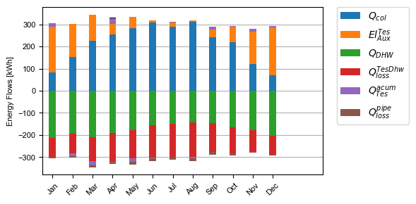
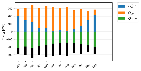
A table with the monthly heat balance. The values are also shown in a plot, in the case of the solar domestic hot water example system this looks like the following:

A electricity balance similar to the heat balance.
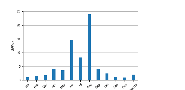
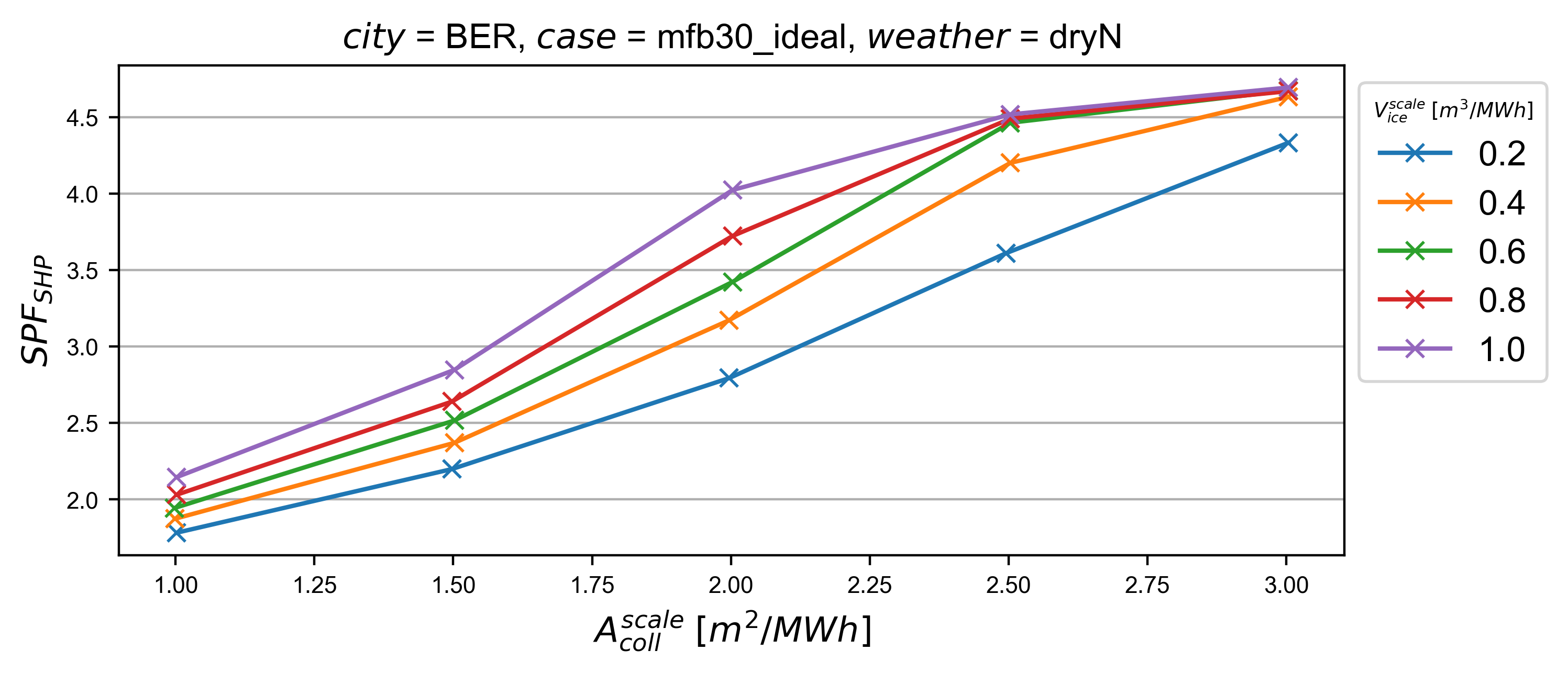
The system seasonal performance factor both in a table and a plot. Again, the SPF plot of the solar domestic hot water system looks like:

Plotting hourly data¶

Note

If an argument in the code excerpts below is set in square brackets, it is optional.

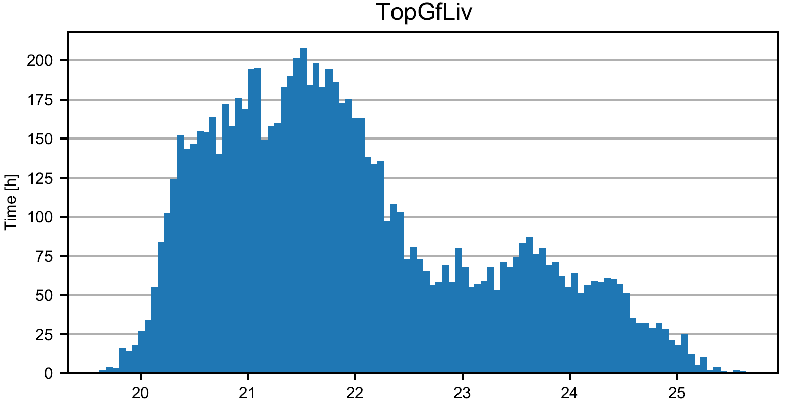
plotT

This generates one or more frequency analysis plots for hourly variables, i.e., bar plots of bandwidth bins for certain values of the respective variables (originally aimed at temperatures, hence the name). It provides an overview over how often a certain value range of a variable appears:

stringArray plotT "hourly variable 1" "hourly variable 2" ...

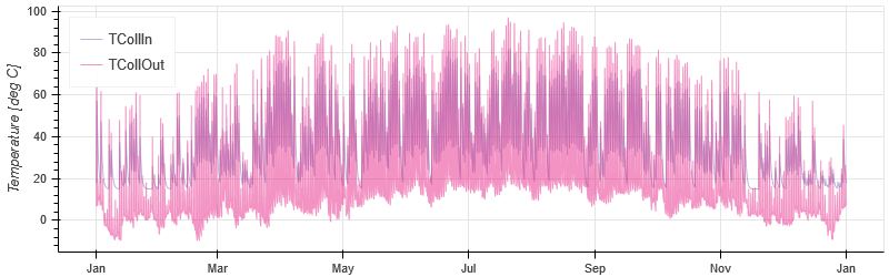
plotHourly

Hourly printed values can be displayed in an interactive HTML plot that is created using the bokeh plotting library.

scatterHourly

Hourly printed values can be displayed as a scatter plot:

stringArray scatterHourly "x_variable" "y_variable"

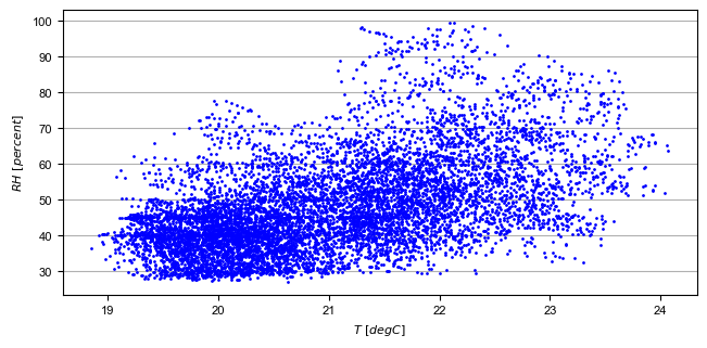
comfortHourly

The hourly printed humidity of a room can be plotted against the hourly printed room temperature and be compared to different comfort norms:

stringArray comfortHourly ["norm"] "temperature_variable" "humidity_variable"

There are two norm boundaries available. The default one (can also be actively called by setting norm to ISO7730) is ISO 7730: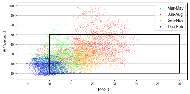

The alternative one is according to this publication and can be employed by setting norm to Dahlheimer: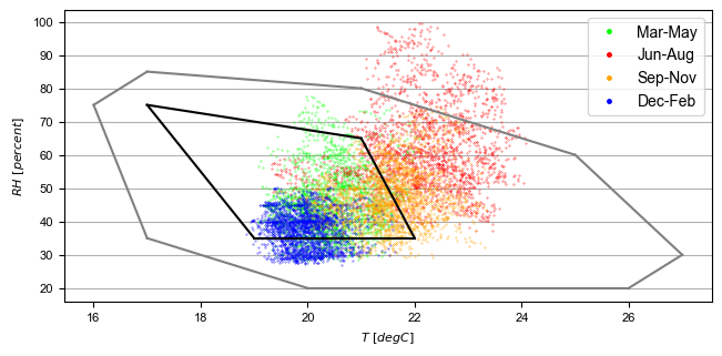

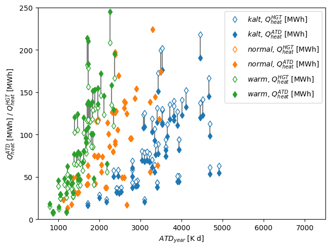
plotHourlyQvsT: Adds a cumulative plot that contains a line for each heat temperature pair given in the string array. Used to show at what temperature levels the heat is released or consumed in different system components. Uses hourly printer files.

Plotting monthly data¶

Note

If an argument in the code excerpts below is set in square brackets, it is optional.

monthlyBars

Plots a monthly bar plot that shows all variables grouped side by side. The name of the pdf to be created needs to specified through pdf name:

stringArray monthlyBars "pdf name" "variable 1" "variable 2" ...

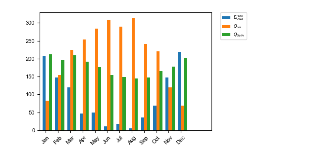
monthlyBalance

Custom monthly balance. The sign of the values can be inverted by adding a - in front of the variable name. If positive and negative values don’t add up to zero, the imbalance is shown as black bars. The name of the pdf to be created needs to be specified through pdf name. When adding the optional style:relative the bars will be shown as values relative to the positive sum of the monthly energy values:

stringArray monthlyBalance "pdf name" ["style:relative"] "variable 1" "variable 2" ...

In the solar domestic hot water example system this can be demonstrated by plotting the two system inputs \(Q_{col}\) and \(El_{Aux}^{Tes}\) and the usable output of the domestic hot water demand. The imbalance in this case are the overall losses of the system.

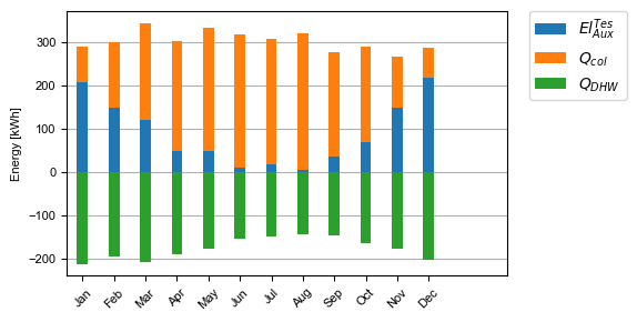
monthlyStackedBar

Similar to the monthlyBalance but without showing the imbalance. The name of the pdf to be created needs to be specified through pdf name:

stringArray monthlyStackedBar "pdf name" "variable 1" "variable 2" ...

Plotting time-step data¶

plotTimestepQvsT: Adds a cumulative plot that contains a line for each heat temperature pair given in the string array. Used to show at what temperature levels the heat is released or consumed in different system componenets. Uses timestep printer files.

Plotting parametric data¶

Note

If an argument in the code excerpts below is set in square brackets, it is optional.

Note

All variables used for the parametric plots need to be saved in the -results.json files.

comparePlot

When processing parametric runs, scalar results of the simulations can be visualized in comparison plots. The first variable of the string array is shown on the x-axis. The second variable is shown on the y-axis. The third is represented as different lines, and the fourth as different marker styles:

stringArray comparePlot "x_variable" "y_variable" ["series 1 variable"] ["series 2 variable"] ["filter1"] ["filter2"] ...

Additionally, you can filter the data that should be plotted by passing in filter expressions for the “filter”s above: only the data taken from -results.json files that match the filter expressions will then be considered. Filter expressions can take the following form:

Equality:

key=value
key=value1|value2|...

For multiple values to be included, they need to be separated by | without spaces. For equalities the values can be numbers or strings, depending on the type of the key.

Inequality:

key>value
key<value
key>=value
key<=value

Logically, for inequalities value needs to be a number.

Ranges:

value1<key<value2
value1<key<=value2
value1<=key<value2
value1<=key<=value2

Ranges need to be specified by < or <= and the values need to be numbers. Note that each key can only be used once, so a range cannot be replaced by two separate inequality statements.

comparePlotConditional (deprecated)

Same as comparePlot, only retained for backwards compatibility. Use comparePlot instead.

comparePlotUncertain

Same as comparePlot but displays uncertain values with error bars:

acrossSetsCalculationsPlot

Has the same basic functionality as acrossSetsCalc, but can plot the results of equations provided:

stringArray plotCalculationsAcrossSets "x_variable" "y_variable" "calculation variable" "equation 1" ["equation 2"] ... ["key 1:value 1"] ["key 2:value 2"] ...

scatterPlot

Generates scatter plots:

stringArray scatterPlot "x_variable" "y_variable" ["series 1 variable"]

When a - is added to y_variable a scatter plot indicating differences is generated:

stringArray scatterPlot "x_variable" "y_variable 1-y_variable 2" ["series 1 variable"]

Example¶

The following processing-configuration file is part of the solar domestic hot water example system:

######### Generic ########################
bool processParallel False
bool processQvsT True
bool cleanModeLatex False
bool forceProcess  True
bool setPrintDataForGle True
bool printData True
bool saveImages True
int reduceCpu 1

######### Time selection ########################
int yearReadedInMonthlyFile -1
int firstMonthUsed 6     # 0=January 1=February 6=July 7=August

############# PATHS ##############################
string latexNames ".\latexNames.json"
string pathBase "C:\Daten\OngoingProject\pytrnsysTest\SolarDHW_newProfile"

############# CALCULATIONS ##############################

calcMonthly fSolarMonthly = Pcoll_kW/Pdhw_kW
calc fSolar = Pcoll_kW_Tot/Pdhw_kW_Tot

calcMonthly solarEffMonthly = PColl_kWm2/IT_Coll_kWm2
calc solarEff = PColl_kWm2_Tot/IT_Coll_kWm2_Tot

############# CUSTOM PLOTS ##############################
stringArray monthlyBars "elSysIn_Q_ElRot"  "qSysIn_Collector" "qSysOut_DhwDemand"
stringArray monthlyBars "solarEffMonthly"
stringArray monthlyBalance "elSysIn_Q_ElRot"  "qSysIn_Collector" "-qSysOut_DhwDemand"
stringArray monthlyStackedBar "elSysIn_Q_ElRot" "qSysIn_Collector" "-qSysOut_DhwDemand"

stringArray plotHourly "Pcoll_kW" "Pdhw_kW" "TCollIn" "TCollOut"  # "effColl" # values to be plotted (hourly)
stringArray plotHourlyQvsT "Pdhw_kW"  "Tdhw" "Pcoll_kW" "TCollOut"

stringArray comparePlot "AcollAp" "fSolar" "volPerM2Col"
stringArray comparePlot "AcollAp" "fSolar" "volPerM2Col"
stringArray comparePlot "AcollAp" "Pdhw_kW_Tot" "volPerM2Col"


############# RESULTS FILES ##############################
stringArray hourlyToCsv "CollectorPower" "IT_Coll_kWm2" "PColl_kWm2"
stringArray results  "AcollAp"  "Vol_Tes1"   "fSolar"  "volPerM2Col"  "Pdhw_kW_Tot" # values to be printed to json